Data Corruption - Part 2 (Digital Degradation)

More causes of bad data...

This series on Data Corruption in Control Systems explores the most common—yet frequently overlooked—problems affecting industrial control system performance and associated data & analytics.

In part 1, we discussed Signal Filtering. In this post (part 2) we cover Digital Resolution & Degradation issues. In part 3, we will cover Input Accuracy & Precision, and in part 4, we will cover Output Device Behaviors & Impacts. 

Data Corruption - Part 2 (Digital Degradation Factors)

In Part 1 of our Data Corruption series, we explored how signal filtering addresses noise at the source—the first critical step in maintaining data integrity.

Now, we'll examine how digital data degrades as it travels through measurement and control systems. Many of the digital degradation errors are small in contrast to the signal noise issues covered previously – but there are a few that can have a big impact on data, control, and safety. In this article we will discuss:

• Timing and synchronization problems
• Resolution and bit-depth degradation, and various comms and programming issues;
• Integer data challenges; 
• System-specific degradation points
• A methodical pathway to identifying and solving data problems 

Let's begin:

1. Timing and Synchronization Problems

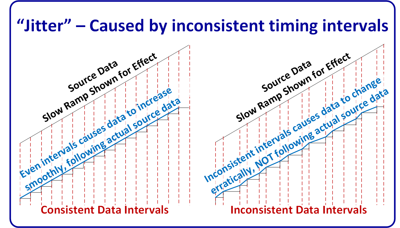
1.1 Network Latency and Jitter

This is one of the more substantial (and more common) issues covered in this article.

Network timing variations can cause the data change rates to appear to change at different rates from reality. This will impact things like PID controls and rate of change calculations among others.

Data or Signal "Jitter" is caused by inconsistent data intervals, which can arise in numerous ways, including; mismatches of real-time sampling rates, update interval settings, comms settings, and they can even vary based on current network traffic.

Though the jitter errors themselves are often small – the effect can be substantial because of how it tricks the system into seeing changes that are faster or slower than reality. Instead of steadily ramping increments that match the real PV from interval to interval, the data PV varies more randomly from the actual value at that moment.

Jitter errors can be especially problematic for:

• High gain PID controllers 
• Controllers using Derivative action
• Loops that have exponential characteristics (DP flow, etc.)
• Loops that have high interactivity or influence with other control loops 
• Analytics that directly or indirectly relate to any of the above

Biggest causes of jitter:

• Using asynchronous / non-deterministic networks or communications 
• Not coordinating system timing blindly using the default IO values for:
  • Sampling Rates
  • AI card Request To Send (RTS), Network Update Time (NUT)
  • Comms timing, scheduling, and prioritization

Note - Jitter is a different type of error from the Aliasing errors discussed in Part 1 (signal filtering). If aliasing errors are not corrected, they will combine with any jitter errors compounding the data problems. 

1.2 Timestamp Mis-alignment Problems

Another closely related problem - Different ICSS system components often use independent timestamp clocks, and these clocks aren't always all synchronized. When they drift by even a few milliseconds or hundreds of milliseconds (which will definitely happen), it can create problems similar to the timing issues covered in section 1.1.

Troubleshooting Challenge: When system clocks drift (up to ±2 minutes/month):

• After 3 months: up to ±6 minute discrepancy between various control system timestamps
• During upset investigation, this can obscure actual sequence of events
• Root cause analysis may incorrectly attribute causality based on misaligned timestamps
• This can often be corrected in various ways, such as use of a master clock or universal timing, depending on control system - but for various reasons (security, etc.), some systems are still likely to be outside the rest of the system and to have timestamp mismatches.

Note - This is not a big factor for plant controls (because the field controllers typically use the live data vs timestamped data – but it can cause data confusion on the analytics and historical side if not factored in (examples: Engineering studies, Forensic analysis, etc.), 

A great solution for system wide timestamp issues is to utilize a GPS sync clock.

Because of arguably excessive costs for memory usage in many historians, the tag count and/or frequency is often extremely limited and not stored at high enough density (frequency) to be of useful in most analytical situations. A 5-minute "snapshot" does little other than provide some potential 'base load' or generic conditional type information. 

2. Resolution and Bit Depth Degradation

2.1 Resolution Mismatch Between Systems

When high-resolution measurements pass through lower-resolution systems, significant information loss occurs (resolution errors creep in). This applies to all digital systems regardless of manufacturer or platform.

Example: A pharmaceutical scale with 24-bit internal resolution (16.7 million steps) is communicating to a control system through a 16-bit Modbus register (65,536 steps). This 8-bit downgrade reduces the data resolution by 256 times! 

For a 100kg range, this reduces precision from 0.006g per step to 1.53g per step—which may result in off-spec products.

If that data is then sent to a high-resolution system, the resolution errors are still embedded from that point downstream. 

It is very common for a plant or facility to purchase a very expensive, high-resolution measurement device (such as scale mentioned above) in hopes of gaining higher accuracy and/or higher resolution data - not realizing that they are passing the data from that expensive 24-bit device through a 16-bit (or lower) bottleneck in the AI card, comms network, program data / tag structure, etc.., or that they have base errors at other points in the system (such AI card, etc) whose 'total errors' are orders of magnitude higher than the input device. 

Unless the full data path is properly reviewed and verified to find weak links, it may not make sense to spend the extra money on that fancier new device.

Note - Once resolution errors are introduced in a data train, there is no way to remove them. 

See the table below for examples of typical bit resolution errors. 

*32-bit floating point provides higher precision for smaller values and lower precision for larger values.

2.2 Non-Aligned Digital Step Increments

Different bit depths create mismatched "staircases" of values, causing measurements to appear irregular even when the underlying phenomenon changes linearly. 

This phenomenon can cause confusion to technicians when performing calibration or verification checks – or to operators when watching the fine changes of a process variable. A person might make slow steady adjustments and see no response, and then suddenly see a change—leading to false assumptions about transmitter health. Or they may spend excessive time, trying to land at an exact target value that is in between the step increments, and therefore impossible to reach.  

Even a 12-bit system (lowest typical resolution) is still a relatively small factor for overall error (about 0.025% of span) – but it should be understood and factored in, because on some systems small errors become big over time (totalizers, etc.); and because of the mistakes they cause in operations and maintenance. 

3. Math and Scaling Problems

In addition to the possibility of incorrectly entered values in scaling parameters or calculations, there are fixed systemic problems that can arise. Let's discuss the main types of data types used and explain the issues for each. 

3.1 Understanding Common Numerical Data Types 

Control systems use several different numerical systems / data types to represent 'analog' numbers. The data type chosen fundamentally affect precision and range. There are others, but we will cover two of the most common ones for explanation of the concepts and potential errors and problems. 

3.2 Floating Point Numbers

IEEE 754 (Float 32): This number system breaks down into:

• Sign bit: Determines whether the number is positive (0) or negative (1)
• Exponent: Represents the power of 2 the number is multiplied by
• Mantissa/Significand: Represents the significant digits of the number

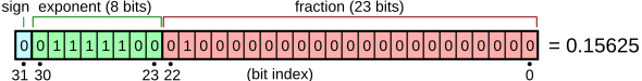
Resolution - An IEEE 754 (Float 32) number has approximately 7 significant decimal digits of resolution (so Pi would show up as 3.141593 for example).

Range - IEEE 754 (Float 32) numbers can represent an enormous range of numbers (from 1.175494 x 10^-38 to 3.402823 x 10³⁸), which makes the particularly useful for calculations and analog processing. 

Trade-offs with Floating Point Numbers: Floating point numbers maintain better relative precision but have non-uniform resolution—smaller values have higher precision than larger values. A 32-bit floating point value provides approximately 7 significant digits of precision. They consume twice as much bandwidth and memory as 16-bit integers - but they provide vastly greater resolution and range and overcome most of the problems inherent to integer numbers (discussed next).  

3.3 Integer numbers: 

Integers: Integer data values have fixed resolution (increment size) across their entire range but are severely limited in both range and precision. We will focus on 16-bit integer data in this description but there are also 8-bit or 32-bit integer data types. 

There are two formats for integer numbers (16-bit shown):

• Unsigned integers: 0-65,535
• Signed integers: -32,768 to +32,767) 

Integer Overflow Faults: When a processor is performing integer calculations, if the result exceeds the range, it will produce an 'overflow' fault - or it could 'wrap over' resulting in grossly inaccurate data and potentially dangerous problems.

Depending on the system and setup, this can cause processor faults that will halt program execution (which results in system shutdown). Great care had to be taken in any calculations to prevent this possibility. 

Integer Truncation: Within integer math, there is no 'rounding' the 'remainders' are simply truncated (or eliminated). For example: 7 ÷ 2 = 3.5 in floating-point - but in integer math it becomes 3! This problem is often missed (or ignored) - but it can have big impact on data quality. 

Integer Scaling & Calculation Problems (& Resolution Loss): Integer calculations sacrifice precision beyond their already limited 16-bit resolution. Division operations truncate fractional parts completely (e.g., 3000/13107 = 0), potentially destroying all scaling information. To preserve maximum resolution, calculations must be strategically ordered—multiply before dividing, use temporary variables for intermediate results, and carefully structure equations to prevent both overflow and significant truncation errors. 

Integer math can (often) introduce errors of up to several percent of span or more - even if arranged correctly in the logic. This issue should be analyzed and factored in on any integer-based calculations. 

4. System-Specific Degradation Points

4.1 Historian Compression Artifacts

Data historians employ compression algorithms that interact poorly with already-quantized data.

Data Integrity Issue: "Swinging door" compression applied to stair-step data:

• Algorithm only stores points needed to reconstruct a trend within tolerance.
• When applied to already-quantized data, may exaggerate step patterns or may 'smooth out' or hide peaks or dips between data points. 
• May create artificial "flat spots" followed by jumps
• Analytics algorithms may detect patterns that don't exist in the process
• This effect is compounded with other errors such as aliasing, bit resolution loss, integer data truncation, etc.. 

4.2 Display and Visualization Distortions

HMI screens are sometimes setup (by design, or per operator selections) to display only the most significant digits or whole numbers of a value, in order to prevent constant ‘flashing’ of changing numbers in the lower digits.

4.3 Engineering Unit Conversions and Math Rounding Errors

Introducing rounded values into logic or code can also introduce errors - and these seemingly small errors can compound and/or produce larger errors than suspected. 

Temperature Conversion Case: Temperature conversion between units:

• Original Kelvin value stored as integer: 293.15K
• Conversion using simplified algorithm: (K - 273) instead of (K - 273.15)
• Result: 20°C instead of 20.15°C (0.075% error)
• These small errors propagate through calculations and compound at each stage.

In short, to maintain maximum precision, use exact values (go out several significant figures beyond what will ever be recorded to ensure it cannot impact the data). If you are multiplying by pi in a calculation for example use 3.1415926535; not the rounded 3.14 value! You are not saving any memory by entering a rounded number - it is still going to consume 16-bits, 32-bits, 64-bits or whatever the data type size is...

4.4 Non-Linear Math – Compounds Errors

Nonlinear or exponential calculations can compound the effect of any errors. 

Example: Differential Pressure to Flow Conversion Errors:
A 0-10 inH₂O DP transmitter used for water flow measurement shows how errors propagate non-linearly:

Note that even a tiny 0.0024% DP error at transmitter results in a 1.2% flow error in the controller data (due to the nonlinear relationship of DP/Flow).

This also illustrates that the programmers and control system design engineers need to think carefully about where they do the math in relation to any errors…

Solving the Problems (Big Picture):

Now that we’ve introduced the first two major groups of problems and errors in the data (and/or control) train, it’s a good time to discuss how to approach the task of identifying and solving the issues. 

Possible Solution: Conduct a methodical study of the error contributions of each item in the data flow path. 

This may sound intimidating - but you may only have 20 to 50 different (important) data flow path variations, and many of them use the same equipment, setups, configs, processor, program layout, etc..

1. Create a block diagram (or better yet, a spreadsheet or equivalent), of each major type of Data Flow Path from the sensor/source to final destinations. Create separate blocks (possibly within other 'container' blocks where appropriate) for the hardware, software, firmware, configuration, program logic, tag structure, comms arrangement, or other functions or details that may potentially cause or impact errors. 
2. Use an iterative process to create a list each potential errors for every item in the data path. 
3. Determine the magnitude of each error (using specs, reference info, maintenance records, analysis, etc..)
4. Analyze the errors and highlight problem areas. If you can, apply cumulative uncertainty calcs to help identify problem areas or areas where extra effort or cost to reduce an error would provide little or no additional value.. For example, a 24-bit scale feeding a 16-bit analog input card per the example in section 2.1 above. 
5. Finally, once you know the total errors / uncertainty of the data - Factor that into decisions and/or fix the problems.

Note – If you approach the task systematically (via spreadsheets, database, or equivalent) you can establish a process that allows for automatic reuse of completed work, and that organizes itself going forward in the engineering lifecycle and which also automatically tallies errors and uncertainties, etc..  

This is just an example approach – The key is to systematically and thoroughly gather the facts, study the problem, and understand what you have - for use in any decisions, controls, or analytics!  

Even the most powerful AI on the planet (5 years from now), will not be capable of knowing what errors are hiding underneath the data you send it.

Good data in = Good decisions = Good results!

Moving Forward

In this series, we have now covered Part 1 - Signal Filtering, and Part 2 - Digital Resolution and Degradation. 

Coming Next: Part 3 (Input Accuracy & Precision) - This is another substantial problem area for overall I&C data, that is frequently overlooked or wrongly assumed to be fine, which can produce bad data right from the source.